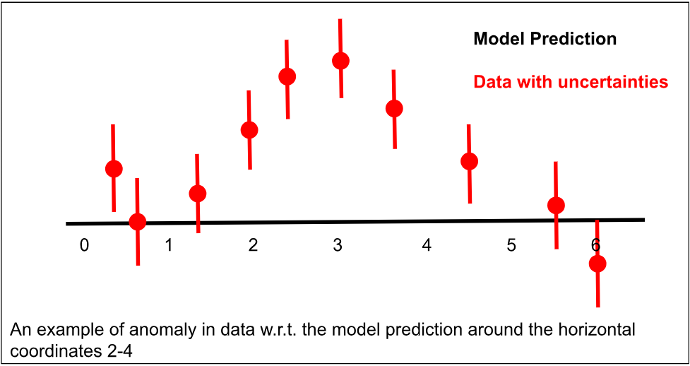
Our present understanding of the Universe is shaped by cosmological observations. Based on a model (built with well established theories + certain supporting assumptions) we match our predictions to the observations and obtain bounds on the model parameters. These bounds refer to the best fit/mean predictions of the model parameters and statistical uncertainties (standard deviation) associated with them. For a model, consistent with the data from an observation, it is expected that the mean model prediction to the observation should be within the reach of a few standard deviations from the observed data. When that does not happen, we term this mismatch as an anomaly in the data. This simple plot describes it.
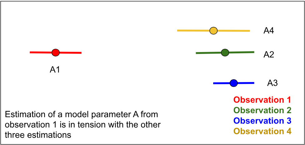
Now, thanks to the different satellite and ground based probes operating at different frequencies, we have access to several observing windows to the Universe. As light travels at a finite speed, through these windows we can witness different stages of the Universe. Now remember that the theoretical model we discussed, provides the origin and evolution of the Universe entirely. Therefore, it is possible to test the model against all observations. We expect that the bounds on the model parameters from different observations lie within the distance of a few standard deviations. Tension between the datasets arise when the distance becomes very large. Here is a representative plot to describe tensions between observations.
Of course, in general, we do not want anomalies and tensions. If the significance of these are high, i.e., when we can rule out statistical fluctuations, we look for two possibilities, namely, systematic errors in analysis and beyond the standard model (new) physics. In many earlier observations or experiments, unaccounted systematic effects were found to be the sources of these anomalies and tensions. On the other hand, since there are also hints of new physics, very often (all the time, for the majority of us) we get excited with the news of such mismatches.
At this point, let’s be more specific about the model. The standard model is based on Einstein’s theory of general relativity (GR). It assumes a homogeneous and isotropic Universe at large scales (supported by observations). Ordinary matter (standard particles with mass), radiation (photon) and unknown type of matter (dark matter, interacts gravitationally) and unknown type of energy (dark energy with negative pressure) are the ingredients of this Universe. Dark matter and dark energy are two very crucial ingredients that we must take seriously as they claim about 95% of the entire energy budget. If we do not take these components into account in our model we can not explain the supernovae luminosities (if you are interested in details, see, Constraining Constituents), rotation curves of galaxies and other observations. Therefore visible matter and radiation as ‘standard model’ ingredients can not fit/address the data well and we find significant anomalies. Therefore once discussed as new physics, dark energy and dark matter become integral parts of today’s standard model. Moreover we assume the negative pressure of the dark energy follows an equation of state given by pressure= – energy density. This particular dark energy is known as the Cosmological Constant (𝜦). With these constituents of the Universe, the background part of the standard model is known as 𝜦 Cold Dark Matter (𝜦CDM) model. I referred to this as the background part, since we have not yet discussed the fluctuations (the structures that we observe in the Universe). These constituents dictate how a homogeneous and isotropic Universe should evolve from an early stage till today. Solving Einstein’s GR, we understand that at very early stages the Universe expanded with deceleration governed by radiation and thereafter by matter. At present we are in a phase of dark energy driven acceleration. We also assume a flat Universe in the standard model (consistent with several observations). Now, let’s understand the fluctuations. The distribution of structures that we observe in the sky such as the galaxies, clusters etc. (with big enough telescopes, obviously) follows a certain pattern, termed as the power spectrum. It tells us how the structures are correlated at different length scales. This power spectrum has evolved since its initial form through the evolution of the Universe and non-linear gravitational collapse. Mathematically we can think of this evolution as a differential equation. The differential equation can be solved with initial conditions. Therefore the natural question is: what was the initial power spectrum of the fluctuations? The seed of these structures has a quantum origin and we need to know the spectrum of these initial (primordial) quantum fluctuations. Without going into the details we can assume the spectrum to have a simple form that can be described with an amplitude and a tilt (power law). So across the length scales if we plot the spectrum it would look like a tilted line (as of now, we do not have any statistically compelling reason to go beyond a tilted line). If we combine these background and initial condition – a flat 𝜦CDM model with power law form of primordial spectrum is known as the standard model of the Universe which is used as the baseline of all our analyses. Therefore an anomaly or tension would mean inconsistencies with respect to the baseline predictions. This baseline model is parametrized with 6 parameters – 4 describing background and 2 describing initial conditions (amplitude and tilt). The 4 background parameters are baryon and cold dark matter densities, today’s Hubble parameter (a measure of how two points in the Universe are receding from each other per unit time per unit distance) and the optical depth (free electron fraction integrated along the line of sight).
We will now be more specific about the observations in question. We will discuss three types of observations:
- The Cosmic Microwave Background (CMB) anisotropy observation from Planck satellite (ESA – Planck: Planck Legacy Archive)
- Large Scale Structure (LSS) surveys from (KiDS: Kilo-Degree Survey and from DES: The Dark Energy Survey
- Today’s Hubble parameter measurement from SHOES-Supernovae, HO, for the Equation of State of Dark energy – NASA/ADS
CMB observation detects photons coming from a time when the Universe was only 380,000 years old (compare it to today’s age of 14 billion years), when the radiation density dropped considerably and matter started to dominate the Universe. These photons have a Uniform temperature of 2.73 Kelvins (how do we know that ? to know in detail, see Fitting FIRAS). Beneath this very uniform temperature, lies tiny fluctuations (see Cosmic Microwave Background Anisotropy to visualize these fluctuations). We can calculate the relation between these fluctuations at different angular scales (which is directly related to the length scales we mentioned before) and average it over the sky – to obtain the angular power spectrum. A precise instrument can probe very small angular scales (to give you an idea, Planck observation used the observed angular power spectrum till 0.07° in their analysis). Ground based observations, such as ACT (Atacama Cosmology Telescope) and SPT (South Pole Telescope) can probe even smaller scales but cannot cover large scales. From the ground, covering full sky is not possible like a satellite probe like Planck. From the largest to a very small angular scale the temperature anisotropy pattern (power spectrum) looks like this:

The red points with bars are the observed data with the standard deviation and the green line is the best fit baseline/standard model prediction. The standard model is doing a remarkable job in fitting that data, isn’t it? Where is the anomaly? Well, if we look at the residual plot (image credit: ESA and the Planck Collaboration) – a plot where best fit standard model has been subtracted from the data to highlight possible anomalies, we notice a pattern between angles 0.2°-0.1° (we can map it to ℓ=800-2000 from the plot above). At larger angular scales we also see other patterns but here we will not talk about those. The pattern between 0.2°-0.1° is oscillatory. Is this pattern an anomaly? We will come to that, but first let’s understand how these patterns arise.
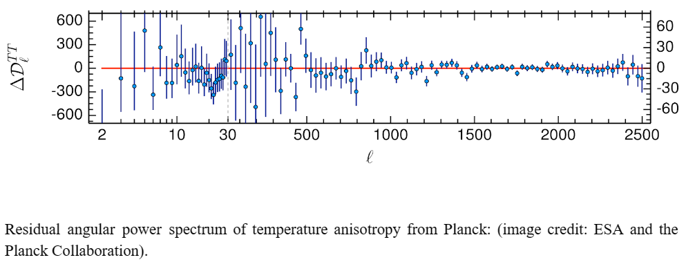
These residual patterns can be generated if we take the map of CMB fluctuations and smudge it. This destroys the signals to some extent by the smearing. This smearing effect is similar to the one produced by weak gravitational lensing of the CMB. I will skip the details but will mention that we have taken the lensing into account in the CMB analysis. That means there is excess smearing. One can show that if an unphysical parameter is introduced called lensing amplitude (Alens), and when it is more than 1 (in standard model, this must be 1), this excess can be explained. Planck analysis in Planck 2018 results – VI. Cosmological parameters | Astronomy & Astrophysics (A&A) the significance of this parameter is reported to be nearly 3 standard deviations (3𝜎). This implies that inclusion of this parameter rejects the theoretical consistency of Alens=1. Since this is an unphysical parameter, we turn to other physical sources to explain this excess smearing. If we relax the assumption that our Universe is flat, then also we can reject the standard model by better addressing the data and a closed Universe picture emerges (see, Planck 2018 results and Planck evidence for a closed Universe and a possible crisis for cosmology | Nature Astronomy). However, the closed Universe picture is also unacceptable – it messes up the initial conditions, and the certain crucial cosmological parameter this picture becomes inconsistent with all other cosmological measurements (in particular, the two other observations that I am going to list).
As I mentioned before, after the radiation dominated the Universe, matter became the most significant component of the Universe. During this epoch, the gravitational attraction brought the particles together and bound them to form structures. A structure (say, galaxy) that is closer to us, distorts the image of a background structure through gravitational lensing (bending of light). Observations of these structures, lensing and their correlations also help us understand the Universe by constraining the model of the Universe. Here I will only talk about a particular parameter called S8 which is a combination of matter density and the 𝜎8. 𝜎8 is related to the amplitude of the matter power spectrum (primordial power spectrum multiplied by a transfer function). It refers to the root mean square fluctuations of matter density within a spherical volume. The radius of that sphere is indicated by the number 8 in certain units. Surveys like the Kilo-Degree Survey and The Dark Energy Survey have observed galaxies over areas of 1500 and 5000 square degrees. Millions of galaxy observations help us in understanding gravitational lensing and galaxy clustering, which, in turn, put bounds on the model parameters. Hence, we get bounds on 𝜎8 and matter density or equivalently on S8. The bounds obtained from KiDS (KiDS-1000 cosmology) and DES (Dark Energy Survey Year 3 Results) are completely consistent. However, the bound derived from Planck CMB data shows an inconsistency at a level of 2 to 3 standard deviations. This we can call a tension of moderate level between CMB and LSS observations.
Now let us discuss physics of (relatively) recent times and of much smaller length scales. We are particularly interested in stars that explode near the end of their life. The luminous explosion is known as Supernova. SNeIa are a particular type of Supernovae that have similar luminosity profiles (how the luminosity behaves over time) and they are found in certain binary systems of stars. Because of the similar profiles, we can use them as scales. Imagine a long football field where we have installed bulbs of the same luminosities. From the intensity of the light we receive from different bulbs, we can understand how far they are. In a similar way, SNeIa help us to understand the distances at much larger length scales. Since the Universe is expanding, they can determine the rate of expansion – today’s Hubble parameter or the Hubble constant. SH0ES team measures the Hubble constant (today’s Hubble parameter) from nearby SNeIa observed by the Hubble Space Telescope over the last few decades. The process of this estimation can be thought of riding three steps/rungs of cosmic distance ladder through the estimation of distance to certain stars exhibiting strong correlation between period and luminosity (standardized cepheid variables) and finding the SNIa in nearby galaxies. The latest SH0ES measurement is discussed in A Comprehensive Measurement of the Local Value of the Hubble Constant. This measurement reports a value of Hubble constant of 73.04 (in units of km/sec/Megaparsecs) about 1.4% uncertainty. Till now I have been avoiding the values of different parameters. Then why is this case different ? Well, let’s have a look at the Planck CMB measurements of the Hubble constant – 67.4 km/sec/Megaparsecs with about 0.7% uncertainty. Here the mismatch points to a severe tension (more than 5 standard deviations). Let me also mention that almost all direct measurements of Hubble constant at late time find higher values than indirect measurements.
These anomalies and tensions certainly bring in the debate between systematics and the new physics, which I will avoid here as this is not the focus of our discussion. I will rather touch upon an interesting correlation between anomalies and tensions that is exciting from the new physics angle. Correlation between anomalies and tension indicates the possibility of a common solution – a solution that solves the anomalies, also solves the tensions.

Several models have been proposed to individually solve the anomalies and tensions. Following the flow of this article let me divide the possible areas of the solution into two parts. primordial Universe and the Universe afterwards. The primordial Universe is characterized by the initial condition, specifically the primordial spectrum of fluctuations. The time afterwards refers to the evolution of the Universe starting from the initial condition. Simply put, the CMB angular power spectrum that I presented from the ESA/Planck collaboration is a matrix multiplication of the primordial spectrum and a transfer function. Remember the primordial spectrum is described by 2 parameters and the transfer function has 4 parameters. Almost all the efforts in the search of new physics to reduce the tensions have been invested in the transfer function part. I am not going to cite any papers here as it is impossible to cite all relevant papers and selective citations is something I would like to avoid. I will discuss some of the papers that I have co-authored. For other efforts in resolving the anomalies and solutions, I request the readers to look at the references cited in these papers.
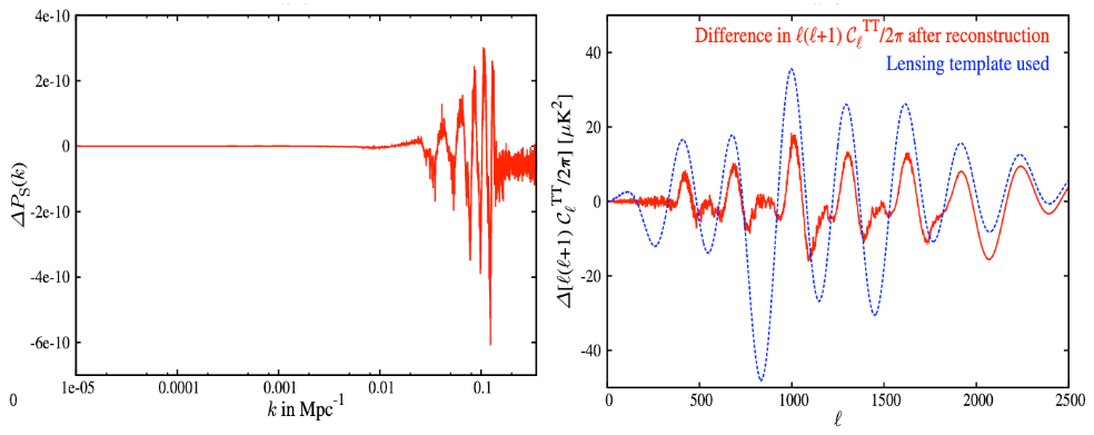
I have started working towards these anomalies starting from the primordial sector. I did not mention ‘tension’ here since initially the works were not dealing with tensions. Initially in the [1406.4827] Primordial power spectrum from Planck, we have worked on a reconstruction of the primordial power spectrum directly from the data. In the last paragraph, I mentioned the CMB power spectrum as a matrix multiplication. Think of our work as a matrix inversion procedure to obtain the initial condition model independently. In section 3.2 of that paper, similarities between oscillations in the primordial spectrum and the CMB lensing have been discussed. In this figure, the left plot shows oscillatory modifications to the primordial spectrum and in the right plot compares its effect (solid red) against the effect of gravitational lensing (blue dashed) in the CMB angular power spectrum. To some extent this type of decaying oscillations seem to be showing effects similar to lensing. In no way this similarity indicates that gravitational lensing is not there. We have detected gravitational lensing earlier and it has to be taken into account in the CMB analysis. I mentioned this similarity as it will come in handy later.
In another work, we attempted a primordial solution to the Hubble constant tension. Do not get confused – the primordial spectrum does not change the value of the Hubble constant. In [1810.08101] Parameter discordance in Planck CMB and low-redshift measurements – we asked the question – ‘is there a power spectrum that, when analyzed with the Planck CMB data, prefers a Hubble constant close to the SH0ES measurements?’ We indeed get a very complicated form of power spectrum. Of course, our attempt to get a robust solution was not successful. We mentioned that ‘it appears to be unnatural to generate the complex form’ of the spectrum. However, we did find that if we find a solution of the problem of Hubble constant through the primordial sector, it will also solve the S8 problem. We also hinted towards a similarity with the lensing effect in relation to this solution.
Afterwards, during the third Planck release, in the paper Planck 2018 results – X. Constraints on inflation | Astronomy & Astrophysics (A&A) – the Planck team discussed that an exponentially decaying sinusoidal oscillation can explain the CMB anomalies around 0.1°-0.2° scales (which is termed as lensing anomalies in many cases because of the excess smoothing of the peaks). Does this ring a bell ? The oscillations we obtained in [1406.4827] had a similar form. So why is this important if we do not want to explain lensing with that ? Simply because we do not have to replace the physics of gravitational lensing but we can explain only the anomalies around 0.1°-0.2° scales which appear as an excess lensing effect. Note that with great flexibility comes more parameters. To introduce oscillations in the primordial spectrum we need 4 extra parameters compared to the standard amplitude and the tilt parameters. We need one parameter to tune the frequency of the oscillations, one for the amplitude, one for the peak position and another for the decay width. Do we have compelling reasons to include 4 extra parameters in our theory? That can be answered with Bayesian evidence, a statistical measure that I will not discuss here.
Let us now return to the idea of a common solution. Can we somehow combine [1406.4827] and [1810.08101] and design a power spectrum through reconstruction to serve as a common solution ? This is exactly what we did in [2201.12000] One spectrum to cure them all: signature from early Universe solves major anomalies and tensions in cosmology. In section 6 of that paper we have discussed how we designed One Spectrum as the common solution to the major anomalies and tensions in Cosmology. The shape of One Spectrum is plotted below in a solid blue line against the standard model spectrum.

We find that the oscillations in the spectrum have a characteristic frequency and with the amplitude peaks at a particular length scale. The P(k) in the plot is simply the primordial spectrum plotted against wavenumbers (inverse of length scale; Mpc is the unit of distance Megaparsecs). This blue colored One Spectrum is beyond the scope of the gray colored standard model spectrum. This One Spectrum, when used as the initial condition:
- It completely cures the anomalies in the Planck temperature anisotropy spectrum around 0.1°-0.2° scales. No excess smoothing is needed to be introduced with the ad-hoc lensing amplitude parameter.
- Of course, the flat Universe becomes completely consistent with the data.
- S8 from CMB becomes completely consistent with the LSS data.
- The mean value of the Hubble constant becomes 70 (it comes midway between standard model CMB analysis and the SH0ES results). It reduces the tension but does not make these two observations completely consistent.
All these results are exciting. However, the question remains. Is this One Spectrum good enough to reject the standard model? To answer this, a parametrization of the spectrum is required. Parametrization here refers to its mapping to an analytical template (expressed by a few parameters) that matches well with One Spectrum. In the same plot above, we show in red color, an analytical template that looks similar to the One Spectrum we designed. When compared with the standard model against the Planck CMB data, we find the model is as good as the standard model. While we get improvement in fit to the data compared to the standard model, the extra parameters adds a penalty (it lowers the preference for the model against simpler models, such as the standard model). Of course, when we perform a joint analysis with CMB, LSS and SH0ES data, our model becomes strongly preferred.
At this point, rather than referring to the One Spectrum and its parametrizations separately, we will call them jointly as the One Spectrum framework. While the framework is supported by several data to certain extents, it is not yet established whether this is the true model of the Universe. The Planck mission has not observed just the temperature anisotropies in the Universe, it has also detected the anisotropies in the photon polarization. In order for the framework to emerge as a new physics, the oscillations should be strongly supported by CMB temperature and polarization observations without adding any other datasets. Note that oscillations in the framework appear at small length scales (0.1°-0.2°), where Planck polarization data can not help because of very high noise. Therefore, we need better small scale polarization data from upcoming observations. The small scale location of the oscillations are also interesting from the galaxy observation. Galaxy power spectrum from Dark Energy Spectroscopic Instrument (DESI), ESA Science & Technology – Euclid, Rubin Observatory will be able to put strong bounds on the parameters in this framework. While we wait for other observations to start, we should ponder over a couple of aspects of this framework:
- Theoretical origin: Anomalies and tensions are the only factors for the development of One Spectrum framework. However, the theoretical origin of these oscillations is one crucial question one can not avoid. In order to hunt for the theoretical origin of this oscillatory power spectrum, we need to work in the possible scenarios of the generation of this initial condition. Inflation (a rapid, near exponential expansion of the Universe before the radiation dominated era) is the most successful candidate theory till now to explain the origin and evolution of the quantum fluctuation in the primordial Universe. In a recent paper [2202.14028] Discordances in cosmology and the violation of slow-roll inflationary dynamics, we demonstrated that a modification of standard inflationary scenarios can generate oscillatory signals similar to the One Spectrum framework. This construction is still phenomenological and is not motivated from high energy theory.
- The signatures that we can analyze with already available data: In the context of CMB, I only discussed the power spectrum. Power spectrum is obtained from the two point correlations of the fluctuations. Bispectrum refers to the three point functions of these fluctuations. Oscillations in the primordial spectrum that we obtained from non standard inflation scenarios give rise to non-negligible bispectrum (to calculate bispectrum from inflationary scenarios, you can use BINGO). This bispectrum can be tested against the CMB bispectrum measured by Planck (see, Planck 2018 results – IX. Constraints on primordial non-Gaussianity | Astronomy & Astrophysics (A&A)). We are working on that.
It will be unfair, and possibly biased too, if I do not mention the other side of the story – the possibilities of One Spectrum framework being ruled out in the future. The origin of this framework is in the CMB anomalies at small scales. If future CMB observations at small scales do not find these anomalies, then the significance of this framework will drop – even if the tensions between different observations persist. One Spectrum originated from CMB anomalies. It cures the CMB small scale anomaly, and in doing so, it reduces the tensions. Therefore if the CMB anomalies are found to be systematic effects, or the future CMB polarization spectrum does not support the oscillations, the model will be less favored if we compare with just the CMB data and forget about the tensions. As of now, it will be safe to treat this framework as a design (possibly the only one) that addresses both CMB anomalies and tensions between CMB and other datasets.
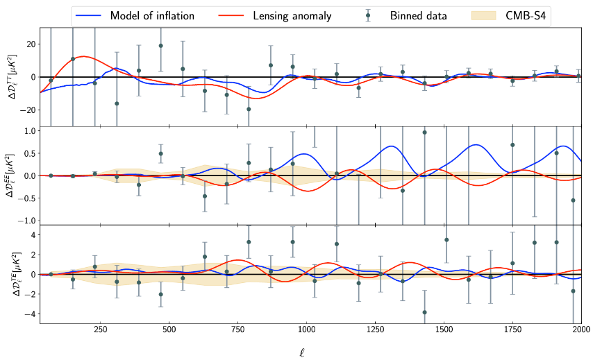
Towards the end, I present a visual forecast to demonstrate what we can expect in the future. With the sensitivities of the proposed/upcoming CMB observations, such as The Simons Observatory, CMB-S4, it is indeed possible to detect or rule out these oscillations in the spectrum. I present one such plot from [2202.14028] where the comparison between Planck and CMB-S4 noise is made in the residual plane of the CMB angular power spectrum. Here both temperature, polarization and their cross-correlation residuals are plotted. The dots and bars are Planck observed data and uncertainties. The yellow band shows the projected uncertainties for CMB-S4. The theoretical inflationary model (blue) from the One Spectrum framework is very similar to the excess lensing (red) as can be seen on the top panel. While both are effectively addressing the anomalies in the temperature data, in the polarization spectrum, their effects are quite opposite (note the mismatch between the red and blue lines in the second panel). As I mentioned earlier, due to high noise (notice the uncertainties in the second panel) the polarization spectrum from Planck is blind to the differences between the standard model (zero line) and red and blue lines. CMB-S4, on the other hand, will clearly identify the differences.
To summarize this article, let me stress again, while the anomalies and tensions in cosmology introduce some hiccups in the study of the Universe, they also create opportunities. The opportunities can come in the form of identifying a new physics or identifying systematic effects. In both ways we explore new avenues. Therefore, simply put, I think anomalies and tensions are exciting and the future observations will offer the litmus test in the understanding of new physics or systematics.